Working with IRIS spectrograph files

In this example, we will showcase how to use irispy-lmsal to open, crop and plot IRIS spectrograph data.

import astropy.units as u
import matplotlib.pyplot as plt
import numpy as np
import pooch
from astropy.coordinates import SkyCoord, SpectralCoord
from sunpy.coordinates.frames import Helioprojective

from irispy.io import read_files

We start with getting the data. This is done by downloading the data from the IRIS archive.

In this case, we will use pooch to keep this example self contained but using your browser will also work.

raster_filename = pooch.retrieve(
    "http://www.lmsal.com/solarsoft/irisa/data/level2_compressed/2018/01/02/20180102_153155_3610108077/iris_l2_20180102_153155_3610108077_raster.tar.gz",
    known_hash="0ec2b7b20757c52b02e0d92c27a5852b6e28759512c3d455f8b6505d4e1f5cd6",
)

Note that when memmap=True, the data values are read from the FITS file directly without the scaling to Float32, the data values are no longer in DN, but in scaled integer units that start at -2$^{16}$/2.

raster = read_files(raster_filename, memmap=True, uncertainty=False)
# Provide an overview of the data
print(raster)
# Will give us all the keys that corresponds to wavelengths.
print(raster.keys())

Collection
----------
Cube keys: ('C II 1336', 'O I 1356', 'Si IV 1394', 'Si IV 1403', '2832', '2814', 'Mg II k 2796')
Number of Cubes: 7
Aligned dimensions: [<Quantity 1. pix> <Quantity 320. pix> <Quantity 548. pix>]
Aligned physical types: [('meta.obs.sequence',), ('custom:pos.helioprojective.lon', 'custom:pos.helioprojective.lat', 'time'), ('custom:pos.helioprojective.lat', 'custom:pos.helioprojective.lon')]

dict_keys(['C II 1336', 'O I 1356', 'Si IV 1394', 'Si IV 1403', '2832', '2814', 'Mg II k 2796'])

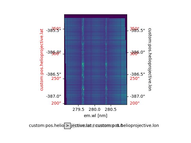
We will now access one wavelength window and plot it.

mg_ii = raster["Mg II k 2796"][0]

plt.figure()
mg_ii.plot()

plt.show()

• 
• 

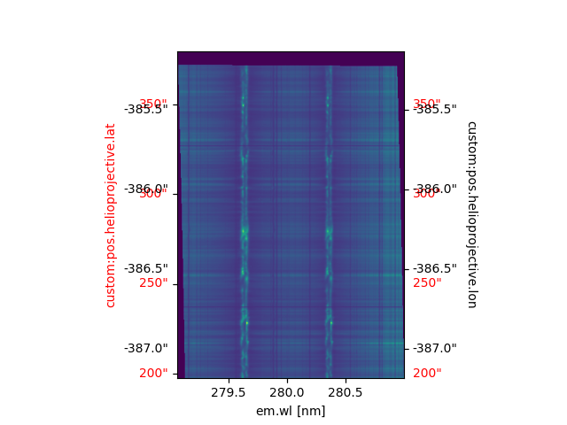
We can index to get the first index and plot it.

plt.figure()
mg_ii[0].plot()

plt.show()

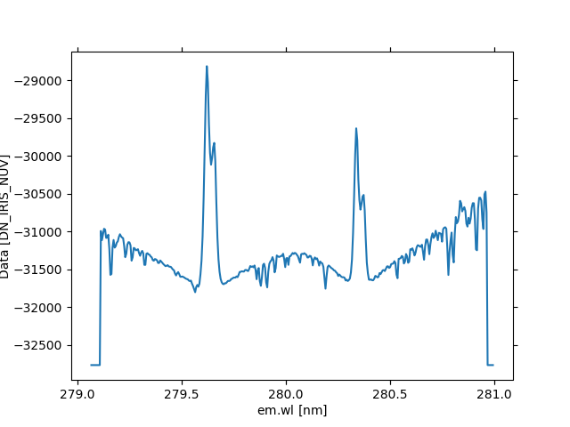
Or we can get the spectrum directly.

plt.figure()
mg_ii[120, 200].plot()

plt.show()

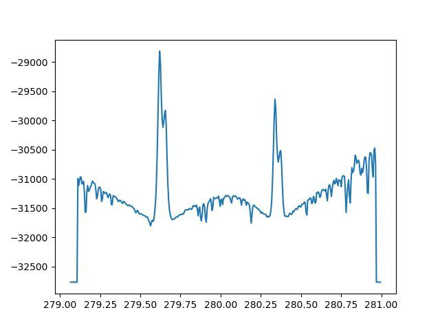
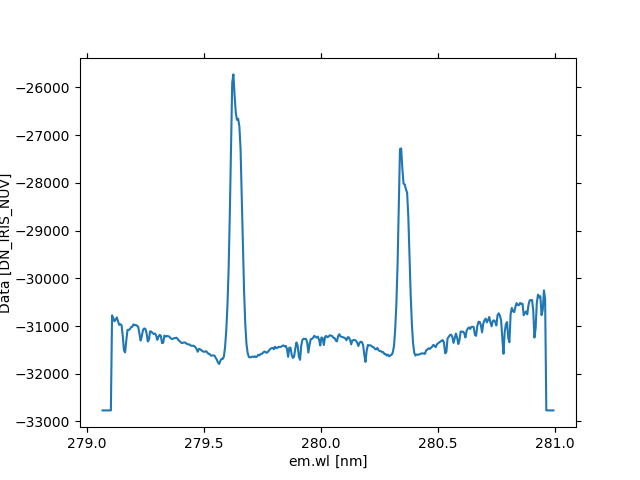
The default plots take the units and labels from the FITS WCS information, and often do not come in the most useful units (e.g. wavelengths in metres). We can read the wavelengths of the Mg window by calling axis_world_coords for wl (wavelength), and redo the plot with a better scale:

(mg_wave,) = mg_ii.axis_world_coords("wl")
mg_wave.to("m")

fig, ax = plt.subplots()
# Here we index the data directly instead of other methods to get access to the data and plot it "raw"
plt.plot(mg_wave.to("nm"), mg_ii.data[120, 200])

plt.show()

/home/docs/checkouts/readthedocs.org/user_builds/irispy-lmsal/conda/stable/lib/python3.10/site-packages/astropy/wcs/wcsapi/fitswcs.py:533: AstropyUserWarning: target cannot be converted to ICRS, so will not be set on SpectralCoord
  warnings.warn(

When we use the underlying data directly, we lose all the metadata and WCS information, so we would suggest not doing it normally but there will be times you will need to do this. If you are unfamiliar with WCS, the following links are quite useful: The base comes from astropy: https://docs.astropy.org/en/stable/wcs/index.html The plotting makes use of WCSAxes: https://docs.astropy.org/en/stable/visualization/wcsaxes/index.html Some of the higher-level utils are via NDCube, e.g. coordinate transformations: https://docs.sunpy.org/projects/ndcube/en/v2.0.0rc2/coordinates.html. We can also improve on the default spectrogram plot by adjusting some options:

plt.figure()
mg_ii[0].plot(aspect="auto", cmap="irissjiNUV")
ax = plt.gca()
ax.coords[0].set_major_formatter("x.x")
ax.coords[0].set_format_unit(u.nm)
ax.set_xlabel("Wavelength (nm)")
ax.set_ylabel("Helioprojective latitude [Solar Y] (arcsec)")
# Remove longitude ticks
ax.coords[2].set_ticks([] * u.degree)

plt.show()

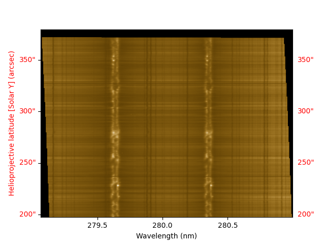
What is the wavelength position that corresponds to Mg II k core (279.63 nm)?

wcs_loc = mg_ii.wcs.world_to_pixel(
    SpectralCoord(279.63, unit=u.nm),
    SkyCoord(0 * u.arcsec, 0 * u.arcsec, frame=Helioprojective),
)
mg_index = int(np.round(wcs_loc[0]))
print(mg_index)

/home/docs/checkouts/readthedocs.org/user_builds/irispy-lmsal/conda/stable/lib/python3.10/site-packages/astropy/wcs/wcsapi/fitswcs.py:533: AstropyUserWarning: target cannot be converted to ICRS, so will not be set on SpectralCoord
  warnings.warn(
/home/docs/checkouts/readthedocs.org/user_builds/irispy-lmsal/conda/stable/lib/python3.10/site-packages/astropy/wcs/wcsapi/fitswcs.py:671: AstropyUserWarning: No observer defined on WCS, SpectralCoord will be converted without any velocity frame change
  warnings.warn(
111

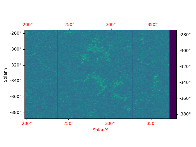
Now we will plot spectroheliogram for Mg II k core wavelength. We can use a new feature in ndcube 2.0 called crop to get this information that will require a SkyCoord and SpectralCoord object from astropy. In this case, we only need to use a SpectralCoord.

lower_corner = [SpectralCoord(280, unit=u.nm), None]
upper_corner = [SpectralCoord(280, unit=u.nm), None]
mg_crop = mg_ii.crop(lower_corner, upper_corner)

ax = mg_crop.plot()
plt.xlabel("Solar X")
plt.ylabel("Solar Y")

plt.show()

Imagine there’s a really cool feature at (-338”, 275”), how can you plot the spectrum at that location?

lower_corner = [None, SkyCoord(-338 * u.arcsec, 275 * u.arcsec, frame=Helioprojective)]
upper_corner = [None, SkyCoord(-338 * u.arcsec, 275 * u.arcsec, frame=Helioprojective)]
mg_ii.crop(lower_corner, upper_corner).plot()

plt.show()

/home/docs/checkouts/readthedocs.org/user_builds/irispy-lmsal/conda/stable/lib/python3.10/site-packages/astropy/wcs/wcsapi/fitswcs.py:533: AstropyUserWarning: target cannot be converted to ICRS, so will not be set on SpectralCoord
  warnings.warn(

Now, you may also be interested in knowing the time that was this observation taken. There is some information in .meta.

print(mg_ii.meta)

SGMeta
------
Observatory:     IRIS
Instrument:      SPEC
Detector:        NUV
Spectral Window: Mg II k 2796
Spectral Range:  [2790.65477674 2809.95345615] Angstrom
Spectral Band:   NUV
Dimensions:      [320, 548, 380]
Date:            2018-01-02T15:31:55.870
OBS ID:          3610108077
OBS Description: Very large dense 320-step raster 105.3x175 320s   Deep x 8 Spatial x

But this is mostly about the observation in general. Times of individual scans are saved in .extra_coords[‘time’]. Getting access to it can be done in the following way:

# The first index is to escape the tuple that ``axis_world_coords`` returns
print(mg_ii.axis_world_coords("time", wcs=mg_ii.extra_coords)[0][0].isot)

2018-01-02T15:31:55.870