Aligning IRIS SJI (rolled) to SDO/AIA

In this example we will show how to align a rolled IRIS dataset to SDO/AIA.

You can get IRIS data with co-aligned SDO data (and more) from https://iris.lmsal.com/search/

import astropy.units as u
import matplotlib.pyplot as plt
import numpy as np
import pooch
import sunpy.map
from aiapy.calibrate import update_pointing
from astropy.coordinates import SkyCoord
from astropy.time import Time, TimeDelta
from astropy.wcs.utils import wcs_to_celestial_frame
from sunpy.net import Fido
from sunpy.net import attrs as a

from irispy.io import read_files
from irispy.obsid import ObsID

We start with getting the data. This is done by downloading the data from the IRIS archive.

In this case, we will use pooch as to keep this example self contained but using your browser will also work.

sji_filename = pooch.retrieve(
    "http://www.lmsal.com/solarsoft/irisa/data/level2_compressed/2014/09/19/20140919_051712_3860608353/iris_l2_20140919_051712_3860608353_SJI_2832_t000.fits.gz",
    known_hash="02a1cdbe2014e24b04ff782dcfdbaf553c5a03404813888ddea8c50a9d6b2630",
)

We will now open the slit-jaw imager (SJI) file we just downloaded.

sji_2832 = read_files(sji_filename)
# Printing will give us an overview of the file.
print(sji_2832)
# ``.meta`` contains the entire FITS header from the primary HDU.
# Since it is very long, we won't actually print it here.

SJICube
-------
Observatory:           IRIS
Instrument:            SJI
Bandpass:              2832.0
Obs. Start:            2014-09-19T05:17:12.610
Obs. End:              2014-09-19T07:14:54.895
Instance Start:        2014-09-19T05:17:31.110
Instance End:          2014-09-19T07:13:24.610
Total Frames in Obs.:  None
IRIS Obs. id:          3860608353
IRIS Obs. Description: Large sit-and-stare 0.3x120 1s  C II   Mg II h/k   Mg II w s Deep x
Axis Types:            [('custom:pos.helioprojective.lon', 'custom:pos.helioprojective.lat', 'time', 'custom:CUSTOM', 'custom:CUSTOM', 'custom:CUSTOM', 'custom:CUSTOM', 'custom:CUSTOM', 'custom:CUSTOM', 'custom:CUSTOM', 'custom:CUSTOM', 'custom:CUSTOM'), ('custom:pos.helioprojective.lon', 'custom:pos.helioprojective.lat'), ('custom:pos.helioprojective.lon', 'custom:pos.helioprojective.lat')]
Roll:                  45.0001
Cube dimensions:       [ 65. 387. 364.] pix

Can’t remember what is OBSID 3860608353? irispy-lmsal has an utility function that will provide more information.

print(ObsID(sji_2832.meta["OBSID"]))

IRIS OBS ID 3860608353
----------------------
Description:                      Large sit-and-stare 0.3x120 1s
SJI filters:                        C II   Mg II h/k   Mg II w s
SJI field of view:                                       120x120
Exposure time:                                               8.0 s
Binning:                               Spatial x 2, Spectral x 2
FUV binning:                         FUV spectrally rebinned x 4
SJI cadence:                                 SJI cadence default
Compression:                                 Default compression
Linelist:                                       Flare linelist 1

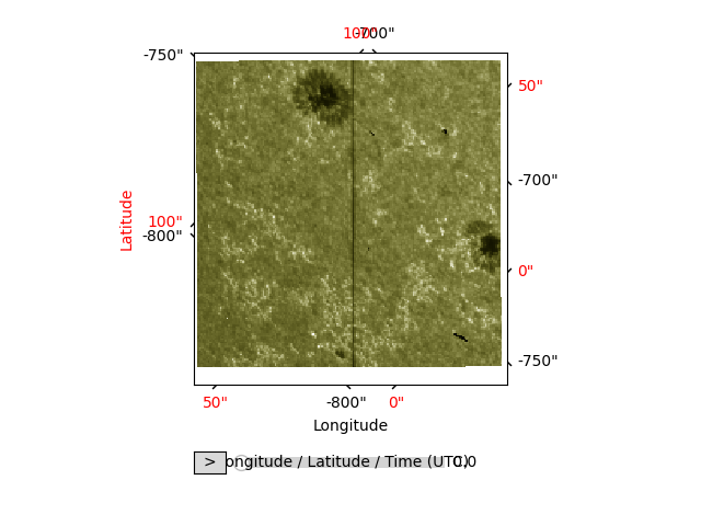
Now, we will plot the SJI. By default, irispy-lmsal will color the spatial axes.

sji_2832.plot()
plt.show()

We also have the option of going directly to an individual scan.

sji_cut = sji_2832[45]
print(sji_cut)

SJICube
-------
Observatory:           IRIS
Instrument:            SJI
Bandpass:              2832.0
Obs. Start:            2014-09-19T05:17:12.610
Obs. End:              2014-09-19T07:14:54.895
Instance Start:        2014-09-19T06:39:00.270
Instance End:          None
Total Frames in Obs.:  None
IRIS Obs. id:          3860608353
IRIS Obs. Description: Large sit-and-stare 0.3x120 1s  C II   Mg II h/k   Mg II w s Deep x
Axis Types:            [('custom:pos.helioprojective.lon', 'custom:pos.helioprojective.lat'), ('custom:pos.helioprojective.lon', 'custom:pos.helioprojective.lat')]
Roll:                  45.0001
Cube dimensions:       [387. 364.] pix

We need to get the coordinate frame for the IRIS data. While this is stored in the WCS, getting a coordinate frame is a little more involved. We will use this to do a cutout later on but for now we will plot it.

sji_frame = wcs_to_celestial_frame(sji_cut.basic_wcs)
bbox = [
    SkyCoord(-750 * u.arcsec, 90 * u.arcsec, frame=sji_frame),
    SkyCoord(-750 * u.arcsec, 95 * u.arcsec, frame=sji_frame),
    SkyCoord(-700 * u.arcsec, 90 * u.arcsec, frame=sji_frame),
    SkyCoord(-700 * u.arcsec, 95 * u.arcsec, frame=sji_frame),
]

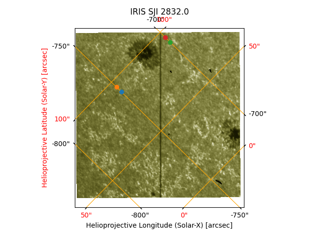
This dataset has a peculiarity: the observation has a 45 degree roll. The image does not have a 45 degree rotation because plotting shows the data in the way they are written in the file. We will a coordinate grid to make this clear. You can also change the axis labels and ticks if you so desire. WCSAxes provides us an API we can use.

plt.figure()
ax = sji_cut.plot()
plt.xlabel("Helioprojective Longitude (Solar-X) [arcsec]")
plt.ylabel("Helioprojective Latitude (Solar-Y) [arcsec]")
plt.title(f"IRIS SJI {sji_2832.meta['TWAVE1']}", pad=20)
ax.coords.grid(color="orange", linestyle="solid")

lon = ax.coords[0]
lat = ax.coords[1]

lon.set_ticklabel_position("all")
lat.set_ticklabel_position("all")
lon.set_axislabel(ax.get_xlabel(), color="black")
lon.set_ticklabel("black")
lat.set_axislabel(ax.get_ylabel(), color="red")
lat.set_ticklabel("red")

# Plot each corner of the box
[ax.plot_coord(coord, "o") for coord in bbox]

plt.show()

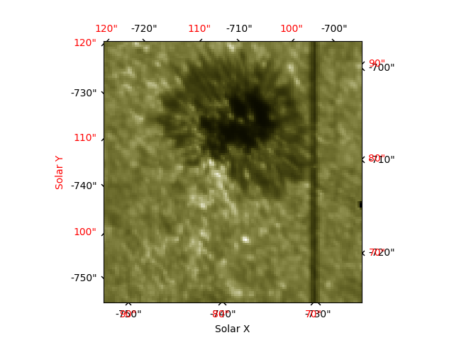
For example, let us cut out the top sunspot. We need to specify the corners for the cut (note the coordinate order is the same as the plotted image). Be aware that crop works in the default N/S frame, so it will crop along those axes where as the data is rotated. You will also need to create a proper bounding box, with 4 corners.

crop will return you the smallest bounding box which contains those 4 points which we can see when we overlay the points we give it.

sji_crop = sji_cut.crop(*bbox)
sji_crop.plot(vmin=0, vmax=5000)
plt.xlabel("Solar X")
plt.ylabel("Solar Y")

plt.show()

We will want to align the data to the AIA. First we will want to pick a timestamp during the observation.

Lets us now find the SJI observation where the time is closest to 06:00 on 2014-09-19.

(time_sji,) = sji_2832.axis_world_coords("time")
time_target = Time("2014-09-19T06:00:00.0")
time_index = np.abs(time_sji - time_target).argmin()
time_stamp = time_sji[time_index].isot
print(time_index, time_stamp)

23 2014-09-19T05:59:10.020

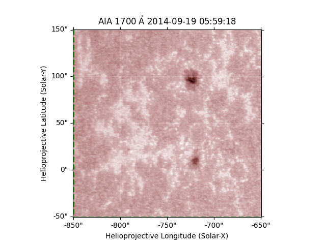
The fact that it is rolled 45 degrees makes manual alignment tricky and will illustrate the usefulness of working with WCS. We will download an AIA 170 nm image from the VSO. Once we have acquired it, we will need to use aiapy to prep this image.

search_results = Fido.search(
    a.Time(time_stamp, Time(time_stamp) + TimeDelta(1 * u.minute), near=time_stamp),
    a.Instrument.aia,
    a.Wavelength(1700 * u.AA),
)
files = Fido.fetch(search_results)
aia_map = sunpy.map.Map(files[0])
aia_map = update_pointing(aia_map)

# You don't need to register AIA images unless you need them aligned to other AIA images.
# otherwise you are degrading the data as the affine transform is not perfect.
# But it is the last step to get a level 1.5 image.
#

Files Downloaded:   0%|          | 0/1 [00:00<?, ?file/s]

aia_lev1_1700a_2014_09_19t05_59_18_71z_image_lev1.fits:   0%|          | 0.00/12.8M [00:00<?, ?B/s]

aia_lev1_1700a_2014_09_19t05_59_18_71z_image_lev1.fits:   0%|          | 1.02k/12.8M [00:00<2:38:15, 1.35kB/s]

aia_lev1_1700a_2014_09_19t05_59_18_71z_image_lev1.fits:  10%|█         | 1.32M/12.8M [00:00<00:05, 2.07MB/s]

aia_lev1_1700a_2014_09_19t05_59_18_71z_image_lev1.fits:  46%|████▋     | 5.94M/12.8M [00:00<00:00, 10.2MB/s]

aia_lev1_1700a_2014_09_19t05_59_18_71z_image_lev1.fits:  86%|████████▋ | 11.1M/12.8M [00:01<00:00, 18.7MB/s]


Files Downloaded: 100%|██████████| 1/1 [00:06<00:00,  6.29s/file]
Files Downloaded: 100%|██████████| 1/1 [00:06<00:00,  6.29s/file]

Now let’s plot the IRIS field of view on the AIA image. This IRIS data has no observer coordinate information irispy-lmsal will set this to be at Earth. This will allow us to transform from IRIS to any another observer.

Using draw_quadrangle(), drawing regions is straightforward.

aia_bottom_left = SkyCoord(-850 * u.arcsec, -50 * u.arcsec, frame=aia_map.coordinate_frame)
aia_top_right = SkyCoord(-650 * u.arcsec, 150 * u.arcsec, frame=aia_map.coordinate_frame)
aia_sub = aia_map.submap(aia_bottom_left, top_right=aia_top_right)

fig = plt.figure()
ax = plt.subplot(projection=aia_sub)
aia_sub.plot()
aia_sub.draw_quadrangle(
    (0, 0) * u.pix,
    width=sji_cut.data.shape[1] * u.pix,
    height=sji_cut.data.shape[0] * u.pix,
    edgecolor="green",
    linestyle="--",
    linewidth=2,
)

plt.show()

# ###############################################################################
# # Now let's plot the IRIS field of view on the AIA image using the information
# # from the WCS coordinates. This IRIS basic WCS has no observer coordinate information
# # so we are just going to pretend it's at AIA for this example.
# # This will allow us to transform from IRIS to SDO/AIA.


# # We have to re-create the coordinate frame.

We have a green square showing the region of the IRIS observation. To work with both IRIS and AIA data, it helps if the image axes are aligned, and for this we need to rotate one of them. We can either rotate SDO/AIA to the IRIS frame, or vice-versa.

We will rotate the AIA data, using reproject_to. As sunpy does not support gWCS, we have to use the basic WCS.

aia_rot = aia_sub.reproject_to(sji_cut.basic_wcs)

# Crop the AIA FOV to match IRIS.
bl = aia_rot.wcs.world_to_pixel(sji_cut.basic_wcs.pixel_to_world(*(0, 0) * u.pix))
tr = aia_rot.wcs.world_to_pixel(
    sji_cut.basic_wcs.pixel_to_world(*(sji_cut.data.shape[0], sji_cut.data.shape[1]) * u.pix),
)

/home/docs/checkouts/readthedocs.org/user_builds/irispy-lmsal/conda/stable/lib/python3.10/site-packages/sunpy/map/mapbase.py:891: SunpyMetadataWarning: Missing metadata for observation time, setting observation time to current time. Set the 'DATE-AVG' FITS keyword to prevent this warning.
  warn_metadata("Missing metadata for observation time, "
INFO: Missing metadata for solar radius: assuming the standard radius of the photosphere. [sunpy.map.mapbase]
INFO: Missing metadata for solar radius: assuming the standard radius of the photosphere. [sunpy.map.mapbase]

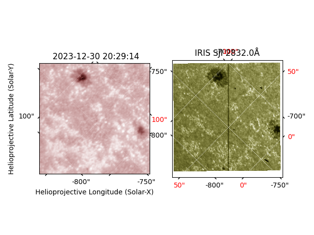
Finally we will plot the results.

fig = plt.figure()
ax1 = fig.add_subplot(1, 2, 1, projection=sji_cut.basic_wcs)
aia_rotate_crop = aia_rot.submap(bl * u.pix, top_right=tr * u.pix)
aia_rotate_crop.plot(axes=ax1, autoalign=True)

ax2 = fig.add_subplot(1, 2, 2, projection=sji_cut.basic_wcs)
sji_cut.plot(axes=ax2, cmap="irissji2832", vmin=0, vmax=4500)
ax2.set_title(f"IRIS SJI {sji_2832.meta['TWAVE1']}Å")
ax2.grid(color="w", ls=":")
ax2.set_xlabel(" ")
ax2.set_ylabel(" ")

plt.show()

INFO: Missing metadata for solar radius: assuming the standard radius of the photosphere. [sunpy.map.mapbase]
INFO: Missing metadata for solar radius: assuming the standard radius of the photosphere. [sunpy.map.mapbase]